A large variety of systems - biological, sociological, technological - can be represented as graphs: nodes representing entities, with connecting edges representing interactions between them. To understand the structure of a network, we may want to detect communities - clusters of nodes that are densely connected to each other. Algorithms such as the Louvain method of community detection involve iteratively re-assigning the nodes to communities, while attempting to optimize the quality of each partition. That is, at each step, the algorithm asks, “How good is this split? How well does it capture the structure of the network?” This measure is called modularity.

The purpose of this post is to provide an intuitive understanding of the modularity measure used in the Louvain method. This post will not discuss how to actually detect communities - instead, it will focus on how to evaluate the quality of a pre-existing partition. Understanding the measure is the first step to optimizing it.

Naive Approach

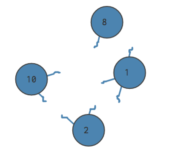
What makes a good partition? Roughly speaking, we care about comparing the density of connections within communities (intra-community) to that between communities (inner-community). If a large fraction of the edges of our graph are contained in the communities, then the communities were “well” chosen. If a small fraction of the edges of our graph are contained in communities, then the communities are “poorly” chosen. Consider this following unweighted, undirected graphs:

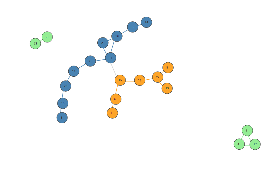
This is a pretty good split! Notice that almost all the edges are green, blue or orange, meaning they exist between nodes who share communities represented by those colors.

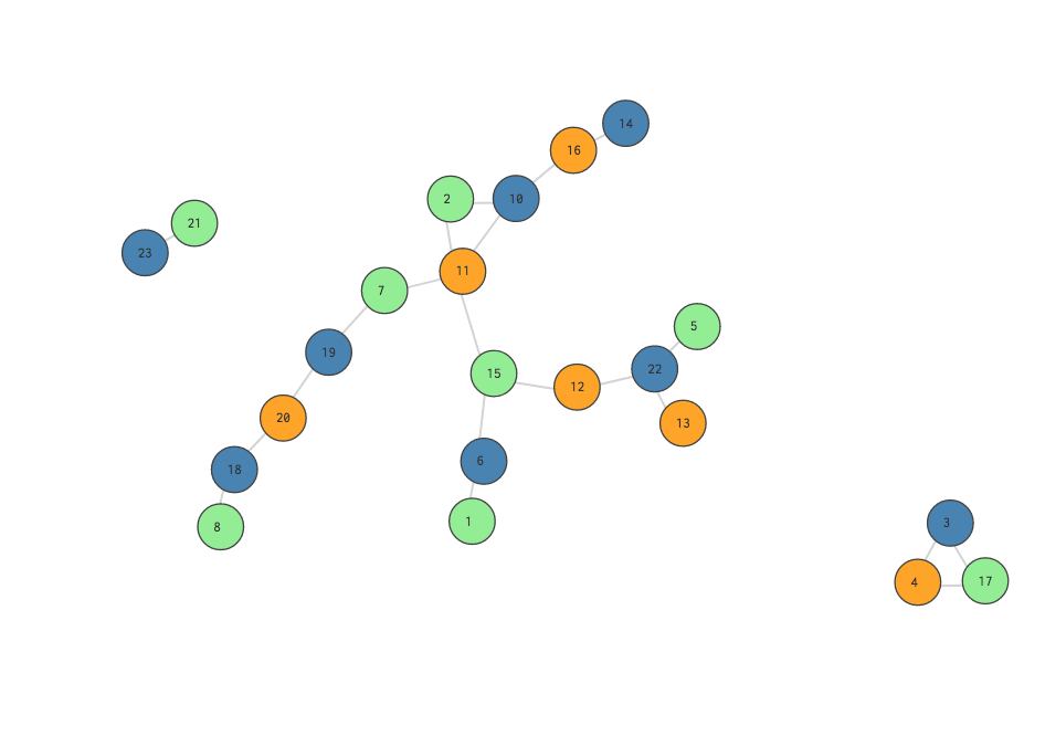
This is a really bad split! Notice that all of the edges are gray, meaning they exist between nodes of different communities.

One naive approach is to simply measure the fraction of the network’s total edges that occur among nodes in the same community. In the visualizations above, this means dividing the colored (green, blue, orange) edges by the total number of edges. A “better” partition will result in a fraction closer to 1. Simple enough, right?

This measure falls short, however, when we consider assigning all nodes to the same community. In this case, 100% of the edges in the network are “intra-community,” but… we only have one community, and where does that get us? We haven’t actually learned anything about our network. Clearly we need a better evaluation function, one that doesn’t reward this “shortcut.”

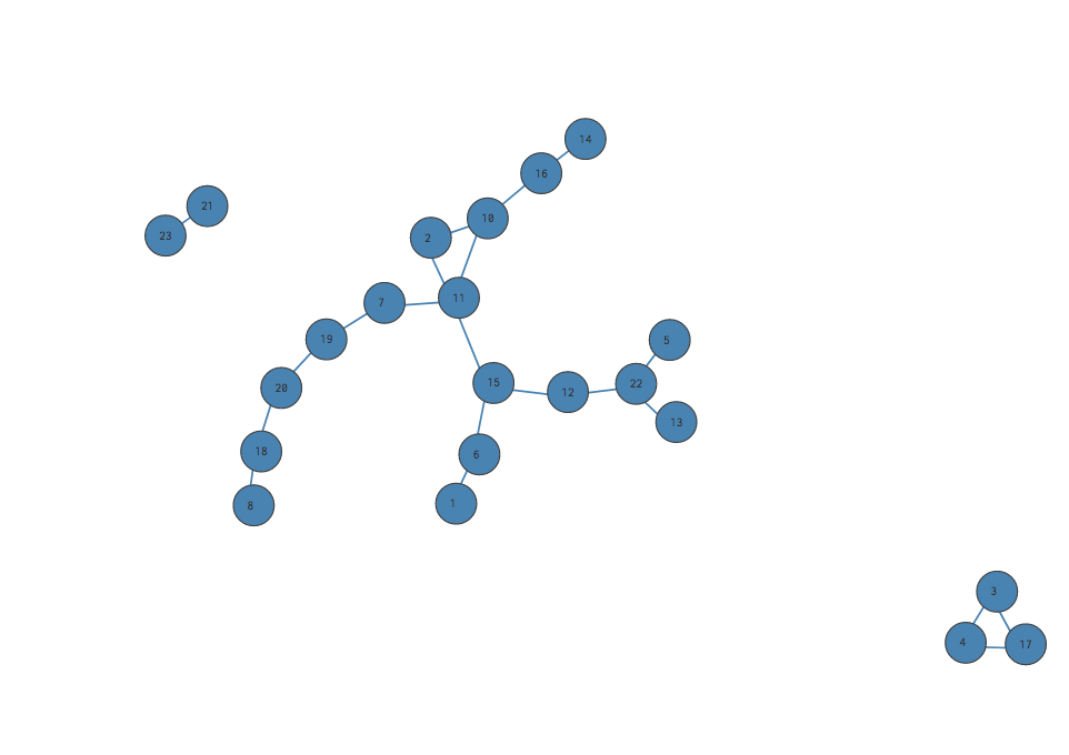
This gets a score of 1 - 100% of the edges are intra-community - but it’s actually a pretty bad split.

Our intuition tells us that assigning all our nodes to a single community isn’t very meaningful, even if it gives us a high fraction of intra-community edges. Why isn’t it meaningful? Because literally any network, no matter its shape, would score 100% on this metric if all its nodes were assigned to one community. If we “rewired” our network again and again, 100 times, 1000 times, each time reconfiguring the nodes with a different set of edges… every single one would get the score 100%.

So… how much of this score is meaningful? None of it. In other words, the entirety of our “good score” occurred due to chance. There was a 100% chance that with this partition, no matter the structure of the graph, all our edges would be intra-, and not inner-, community. The fact that this particular graph got a score of 1, tells us nothing about the graph itself.

So we need an approach that acknowledges - and removes - the effect of chance… one that lets us focus on the part of the modularity score that is due to our graph’s unique structure.

The Null Model

We can formalize this insight by generating a null model of our graph - the “average” of a bunch of random “re-wirings” of our nodes. Then, every time we score our graph (calculating the fraction of intra-community edges out of total edges), we can subtract from it the score - calculated the same way - for the null model. This leaves us with only the part of the original score that is “meaningful” - the part that doesn’t occur due to chance.

---

Given a partition…

modularity =

(weight* of intra-community edges of graph / weight of all edges of graph) -

(weight of intra-community edges in null model / weight of all edges in null model)

*In this definition, we refer to the “weight” of the edges. In an unweighted graph, the “weight” will always be 1. The null model, however, will have edges with fractional weights, which represent the probability of such an edge existing.

---

The null model should have the following characteristics:

• (1) The total weight of the edges should be the same as that of the original graph.
• (2) Each node should have the same degree - that is, the total weight of its edges should reman the same - as in the original graph.
• (3) The null model should represent the average of a large number of graphs randomly created according to the above guidelines.

Guideline (2) is important because it allow us, in our scoring, to acknowledge that the “meaningulfness” of an intra-community edge depends on whether its nodes have many or few connections with other nodes in the original graph. A highly connected node is relatively likely to randomly have an edge with a neighbor in the same community - so the existence of such an edge should not contribute greatly to the modularity score. On the other hand, a node with few connections is relatively unlikely to randomly have an edge with a node in the same community. If it does, our community assignation has probably captured something important about the structure of our network, and our overall modularity score should increase significantly. By maintaining the degree of each node in the null model, we can hold onto these distinctions.

Generating the Null Model

Generating our null model is pretty simple. We have a bunch of nodes that need to be rewired to other nodes, each node maintaining its own degree. While our original graph is unweighted, we can now use weighted edges to accomplish this configuration.

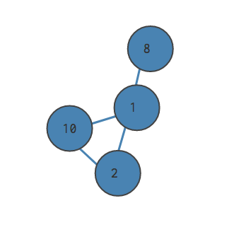
Let’s say our graph has 4 edges. We cut each edge in half, letting our nodes float free. There are now (2 * 4 = 8) “edge stubs.” Some nodes have more stubs than others.

For each distinct pair of nodes in the community, we consider the likelihood of randomly selecting an “edge stub” from the first node out of all the edge stubs. (That is, the number of edge stubs coming from that node, divided by the total number of edge stubs.) Nodes with more connections in the original graph will be more likely to have one of their edge stubs chosen. We then multiply this by the likelihood of selecting an edge stub from the second node, calculated similarly. The probability that we’d selected a stub from node A and the probability that we would select an edge stub from node B is the probability that we would create an edge between them - and this fraction becomes the weight of the edge in the null model.

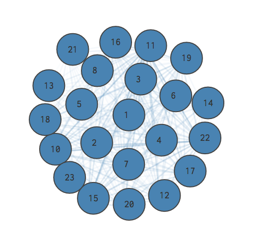
Here is the null model of the larger graph we explored above. The opacity of an edge represents its weight; more opaque lines represent edges with greater weight. A greater weight means the edge is more likely to exist when the graph is “randomly” re-wired.

Does It Work?

To evaluate our measure of modularity, consider the following cases:

• All the nodes are placed in the same community. As discussed above, we get a score of 0.

• The null model predicts some fraction of intra-community edges given this partition; the number of intra-community edges in our real graph is much greater. We get a score above 0, approaching 1 as the difference increases.

• The null model predicts some fraction of intra-community edges given this partition; the number of intra-community edges in our real graph is much smaller. We get a score below 0, approaching -1 as the difference increases.

All of this leaves us with a meaningful measure of modularity! At the “center” of our score range is indecision - placing all the nodes in one community. The more we improve on this partition - by recognizing the “unlikely” intra-community edges, the ones that didn’t just happen due to chance - the closer our score gets to 1.

---

Pssst, I didn’t make this stuff up! You can read more, and see the mathematical notation, here and here.